Usage

Calculation of IBP Index

To calculate the IBP index use ibpmodel.ibpforward.calculateIBPindex() function. It returns a pandas.DataFrame:

>>> from ibpmodel import calculateIBPindex
>>> calculateIBPindex(day_month=15, longitude=0, local_time=20.9, f107=150)
   Doy  Month  Lon    LT  F10.7     IBP
0   15      1    0  20.9    150  0.4332

>>> from ibpmodel import calculateIBPindex
>>> calculateIBPindex(day_month=['Jan','Feb','Mar'], local_time=22)
     Doy  Month  Lon  LT  F10.7     IBP
0     15      1 -180  22    150  0.0700
1     15      1 -175  22    150  0.0699
2     15      1 -170  22    150  0.0690
3     15      1 -165  22    150  0.0687
4     15      1 -160  22    150  0.0726
..   ...    ...  ...  ..    ...     ...
211   74      3  155  22    150  0.2462
212   74      3  160  22    150  0.2460
213   74      3  165  22    150  0.2482
214   74      3  170  22    150  0.2511
215   74      3  175  22    150  0.2533

[216 rows x 6 columns]

>>> from ibpmodel import calculateIBPindex
>>> calculateIBPindex(day_month=[1,15,31], longitude=[-170,175,170], local_time=0, f107=120)
   Doy  Month  Lon  LT  F10.7     IBP
0    1      1 -170   0    120  0.0277
1    1      1  175   0    120  0.0260
2    1      1  170   0    120  0.0256
3   15      1 -170   0    120  0.0306
4   15      1  175   0    120  0.0288
5   15      1  170   0    120  0.0283
6   31      1 -170   0    120  0.0390
7   31      1  175   0    120  0.0366
8   31      1  170   0    120  0.0361

With electron density

/home/docs/checkouts/readthedocs.org/user_builds/ibp-model/envs/v2.0.0/lib/python3.12/site-packages/sklearn/base.py:440: InconsistentVersionWarning: Trying to unpickle estimator StandardScaler from version 1.8.0 when using version 1.7.0. This might lead to breaking code or invalid results. Use at your own risk. For more info please refer to:
https://scikit-learn.org/stable/model_persistence.html#security-maintainability-limitations
  warnings.warn(

Plotting probability

There are two functions to plot IBP index. function ibpmodel.ibpforward.plotIBPindex() and ibpmodel.ibpforward.plotButterflyData(). By default, the plot is displayed immediately. If you want to make changes or additions, the parameter getFig must be set equal to True. Then you get matplat.axis as return value:

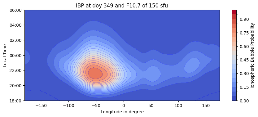
>>> import ibpmodel as ibp
>>> ibp.plotIBPindex(doy=349)

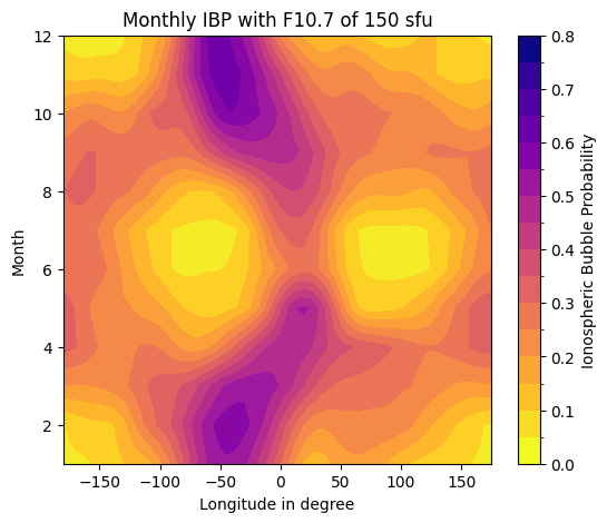
>>> ibp.plotButterflyData(f107=150)

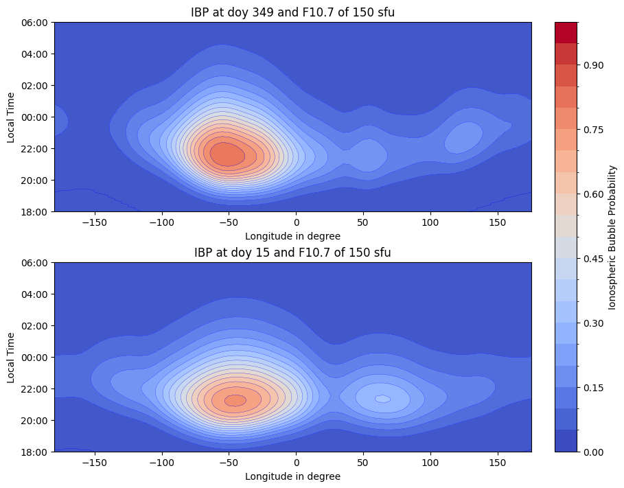
>>> import ibpmodel as ibp
>>> import matplotlib.pyplot as plt
>>> doys = [349, 15]
>>> fig, axes = plt.subplots(len(doys),1, layout='constrained',figsize=(9, 7))
>>> for d, ax in zip(doys, axes):
...     ax, scalarmap = ibp.plotIBPindex(d, ax=ax)
>>> ibp.ibpforward.setcolorbar(scalarmap, fig, axes, fraction=0.05)
>>> plt.show()

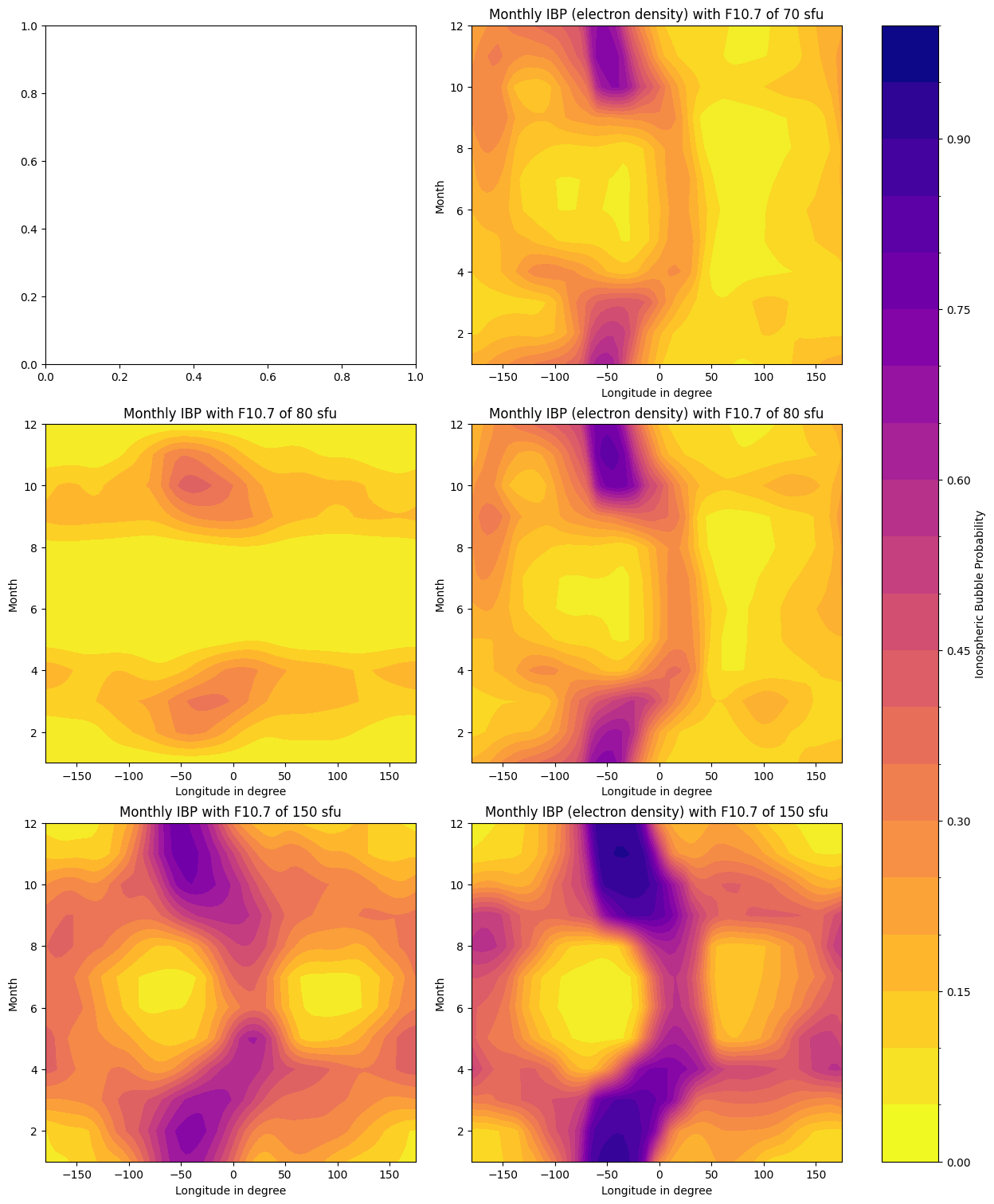
Plotting of magnetic and electron density Model

>>> solar_values = [70, 80, 150]
>>> elecD = [False, True]
>>> fig_bfly, axes_bfly = plt.subplots(len(solar_values), len(elecD), layout='constrained',figsize=(12.4, 5*len(solar_values)))
>>> for axes, so in zip(axes_bfly, solar_values):
...      for b, ax in zip(elecD, axes):
...      try:
...         ax, scalarmap = ibp.plotButterflyData(so, ax=ax, elecDensity=b)
...      except:
...         print(f"Not possible with F10.7 of {so} sfu!")
>>> ibp.ibpforward.setcolorbar(scalarmap, fig_bfly, axes_bfly)
>>> plt.show()

Read coefficient file

You can load the coefficient file. ibpmodel.ibpcalc.read_model_file():

>>> from ibpmodel import read_model_file
>>> c = read_model_file()
>>> c.keys()
dict_keys(['Parameters', 'Intensity', 'Monthly_LT_Shift', 'Density_Estimators', 'Density_Estimator_Lons'])
>>> 
>>> c['Intensity']
array([ -22.34634838,  -11.17710961,   70.04849368,    7.0684529 ,
       -164.54246628])