Usage

Calculation of IBP Index

To calculate the IBP index use ibpmodel.ibpforward.calculateIBPindex() function. It returns a pandas.DataFrame:

For magnetic (dB) model

>>> from ibpmodel import calculateIBPindex
>>> calculateIBPindex(day_month=15, longitude=0, local_time=20.9, f107=150)

>>> from ibpmodel import calculateIBPindex
>>> calculateIBPindex(day_month=[1,15,31], longitude=[-170,175,170], local_time=0, f107=120)

Instead of day of the year, the IBP index for a particular month can be calculated by entering the first three letters of that month as a string input to the variable day_month as shown in the example below. With this choice, the IBP index will be calculated for the median day of the chosen month. Check the function description for more details:

>>> from ibpmodel import calculateIBPindex
>>> calculateIBPindex(day_month=['Jan'], local_time=22)

For electron density (Ne) model

>>> from ibpmodel import calculateIBPindex
>>> calculateIBPindex(day_month=['Nov','Dec'], longitude=-160, local_time=22, elecDensity=True)

Plotting probability

There are two functions to plot IBP index. function ibpmodel.ibpforward.plotIBPindex() and ibpmodel.ibpforward.plotButterflyData(). By default, the plot is displayed immediately. If you want to make changes or additions, the parameter getFig must be set equal to True. Then you get matplat.axis as return value:

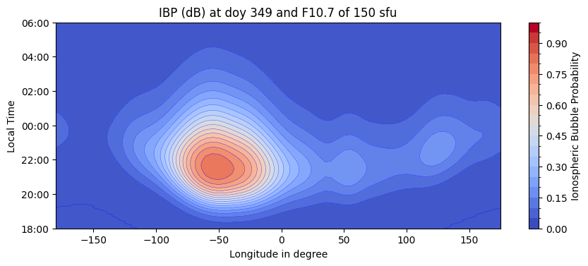
For magnetic (dB) model

>>> import ibpmodel as ibp
>>> ibp.plotIBPindex(doy=349)

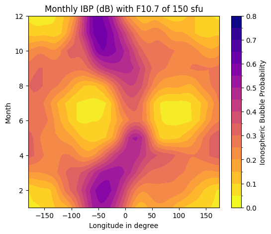
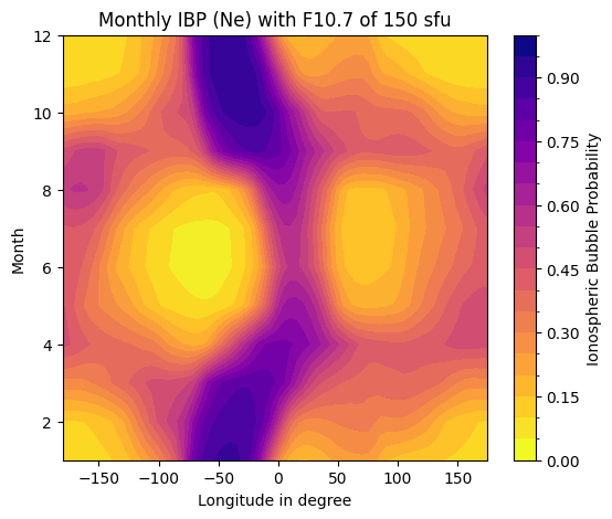
Contour plot of the IBP index for the given day

>>> ibp.plotButterflyData(f107=150)

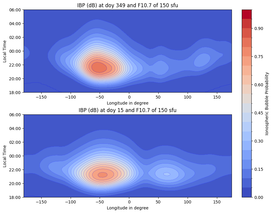
Contour plot of result from function ButterflyData()

>>> import ibpmodel as ibp
>>> import matplotlib.pyplot as plt
>>> doys = [349, 15]
>>> fig, axes = plt.subplots(len(doys),1, layout='constrained',figsize=(9, 7))
>>> for d, ax in zip(doys, axes):
...     ax, scalarmap = ibp.plotIBPindex(d, ax=ax)
>>> ibp.ibpforward.setcolorbar(scalarmap, fig, axes, fraction=0.05)
>>> plt.show()

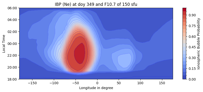
For electron density (Ne) model

>>> import ibpmodel as ibp
>>> ibp.plotIBPindex(doy=349,elecDensity=True)

>>> ibp.plotButterflyData(f107=150,elecDensity=True)

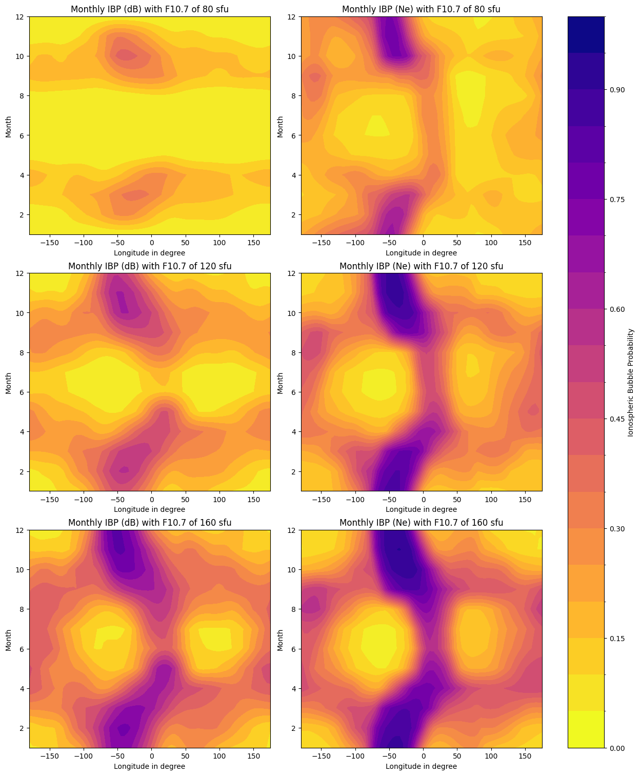
Plotting of magnetic and electron density Models

>>> solar_values = [80, 120, 160]
>>> elecD = [False, True]
>>> fig_bfly, axes_bfly = plt.subplots(len(solar_values), len(elecD), layout='constrained',figsize=(12.4, 5*len(solar_values)))
>>> for axes, so in zip(axes_bfly, solar_values):
...     for b, ax in zip(elecD, axes):
...         ax, scalarmap = ibp.plotButterflyData(so, ax=ax, elecDensity=b)
>>> ibp.ibpforward.setcolorbar(scalarmap, fig_bfly, axes_bfly)
>>> plt.show()

Read coefficient file

You can load the coefficient file. ibpmodel.ibpcalc.read_model_file():

>>> from ibpmodel import read_model_file
>>> c = read_model_file()
>>> c.keys()

>>> c['Intensity']